Don't you (forget about me)

M. Sc. Julia Mausz, Application Scientist, Gatan/EDAX

EDAX^® APEX™ includes a variety of tools and features that can help researchers perform qualitative and quantitative elemental analyses. After all, no one wants to misinterpret measured results because they failed to spot an artifact in a spectrum or missed an element that was there all along.

With a little help from my friends

Luckily, APEX includes plenty of tools to support users, so interpreting your EDS data doesn’t have to feel like walking 500 miles. With a little help from my friends, I’d like to show that performing qualitative and quantitative elemental analyses with APEX software for energy dispersive x-ray spectroscopy (EDS) is both straightforward and reliable.

In EDS spectral analysis, the net intensity of characteristic x-rays from an identified element is calculated after background subtraction and mathematical deconvolution of the peaks. This allows the individual contributions to be assigned to their respective elements.

However, for the software to perform this deconvolution correctly, it must know all the elements present in the sample. When the user does not know an element is there, the deconvolution alone can’t solve the mystery.

This is where spectrum reconstruction comes in handy.

Aside from deconvolving the measured data, APEX calculates a theoretical (under ideal conditions) based on the elements currently selected and microscope accelerating voltage. Comparing this reconstruction with the measured spectrum provides immediate visual feedback on how well your proposed elemental composition explains the data. Mismatches can point toward unidentified elements or other sources of deviation, such as surface topography, sample preparation, or charging.

The software makes the comparison easy to follow using distinct visual indicators: 
Red: Measured EDS data
Blue: Background (uncharacteristic Bremsstrahlung x-rays)
Turquoise: Calculated reconstruction

In Figure 1, the system reconstruction precisely matches the expected peak positions, intensities, and widths of Fe-Kα, Ni-Kα, and Cr-Kα. However, when only chromium is selected (Figure 1a), the expected intensity of Cr-Kβ does not match the EDS data, as indicated by the red arrow. Something is missing.

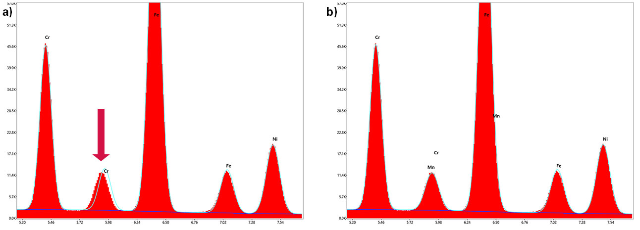
Figure 1. Overview of EDS data (red), reconstruction (turquoise), and background (blue) with a) Cr and b) Cr and Mn.

Taking a closer look at Cr-Kβ, the reconstructed spectrum matches the measured data more accurately when manganese is added, as indicated by the green arrow. Because the reconstruction updates as elements are added or removed, you can immediately see how each change affects the agreement between the measured and reconstructed spectra.

In other words, the reconstruction removes the guesswork and can help point you in the right direction.

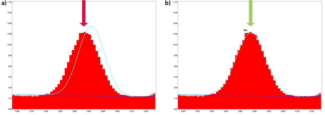
Figure 2. EDS data (red), reconstruction (turquoise), and background (blue) with a) Cr and b) Cr and Mn.

I can see clearly now

Of course, analysts shouldn’t blindly add elements just to force a higher similarity between data and reconstruction. Instead, use this reconstruction strategically as visual feedback to guide your peak identification. The easiest way to confirm that manganese is really present is wavelength dispersive spectroscopy (WDS). With the WDS, I can see clearly now, that the overlapping peak contains contributions from both Mn-Kα and Cr-Kβ.

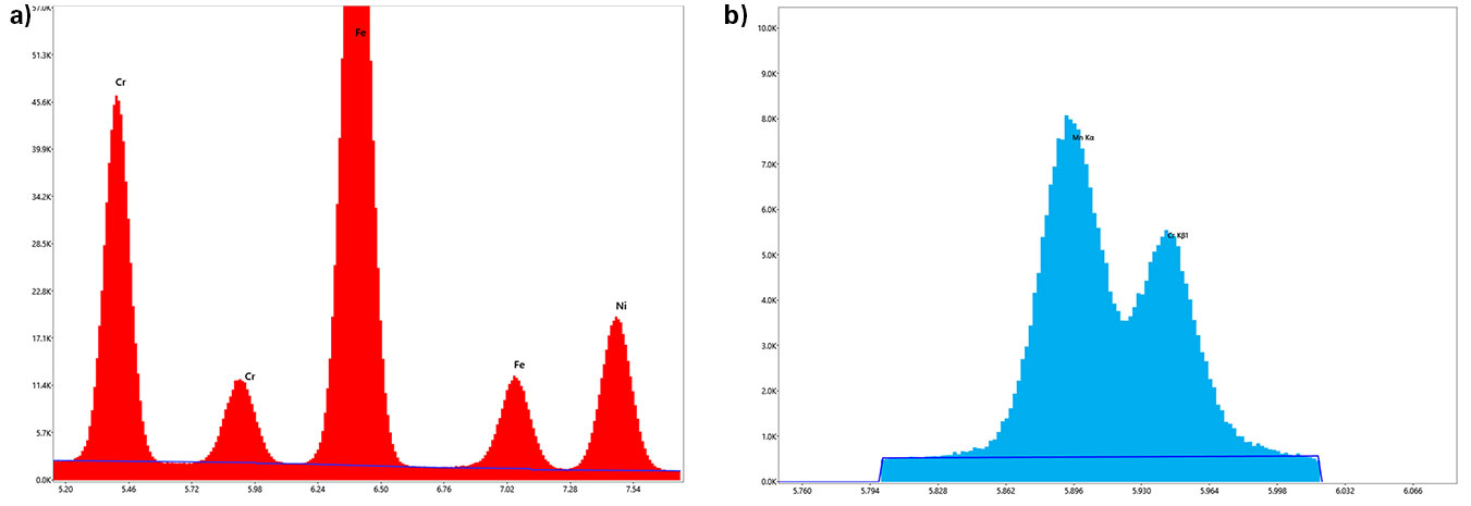
Figure 3. a) EDS without reconstruction and b) confirmation of Mn and Cr presence with WDS.

Smooth operator

A smooth operator knows that accurate element identification also means recognizing artifacts.

Beyond displaying raw spectra, APEX can help identify tricky artifacts like escape and pile-up peaks. Figure 4 illustrates the effect of escape peaks on the raw EDS data and shows the spectrum following escape-peak correction. Correcting for these artifacts helps prevent a peak that isn’t really an element from masquerading as one.

You could say APEX makes those escape peaks disappear with an invisible touch.

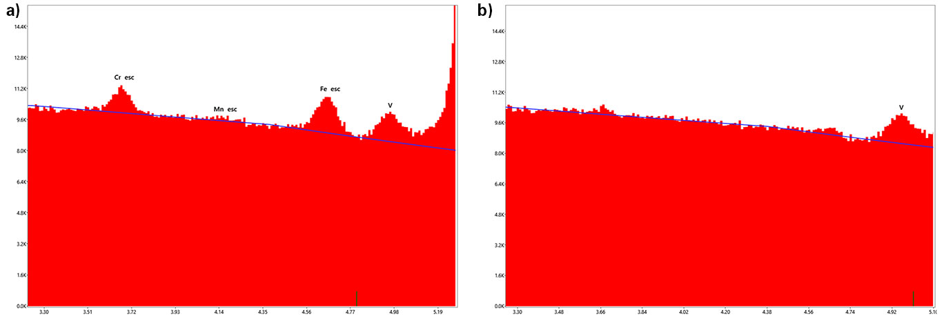
Figure 4. a) Raw EDS data and b) escape peak corrected data.

Blinded by the light?

Sometimes the EDS gets blinded by the light when pile-up or sum peak artifacts appear in the spectrum.

These features can be labeled and estimated based on the elements present, count rate, and amplification time. Accounting for their contribution in the reconstruction helps reassure the user that these peaks do not necessarily represent additional elements.

The individual contribution of the pile up distribution can also be displayed, as shown by the yellow curve at the bottom of Figure 5. This makes it easier to understand where the unexpected intensity is coming from rather than adding another element to the list.

It's a kind of magic

Spectrum reconstruction, artifact identification, escape-peak correction, and complementary analysis with WDS are all tools that can help you look beyond the obvious peaks and build greater confidence in your EDS results.

Once you incorporate these tools into your routine workflow, it’s a kind of magic how much easier it becomes to spot missing elements, understand unexpected peaks, and avoid potential misidentifications.

Hopefully, this blog not only helps improve your EDS analysis, but also inspires you to revisit a few songs you may have forgotten about.

And whatever you do, don’t you forget about them.

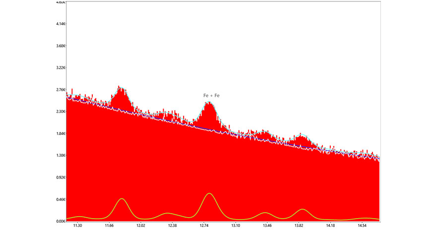
Figure 5. EDS with labeled sum peak and consideration of the pile up distribution (yellow) in the reconstruction.