Extensible real-time data processing with Python in DigitalMicrograph

Modern electron microscopy is often data intensive. Cameras and other detectors have become much faster and sometimes larger than they were a decade ago. In-situ experiments with continuous data acquisition increase the data volume further. In-situ experiments may require decisions where the next experimental step is determined by the changes observed in the microscope. However, these changes are not always apparent from the default live view displayed in real-time. Given the large data volume, it is quite valuable to have the flexibility to process and visualize data in various ways in real-time to understand the changes occurring in the sample. This enables informed decision-making.

For many years Gatan has supported live data processing via our scripting language and the “live view” window, which makes real data (with full resolution and bit depth) available to the user (sometimes at a lower framerate than the camera writes to disk). Gatan recently introduced Python integration in DigitalMicrograph^®. This live processing should be more accessible to researchers since many more people know the Python language. More info on getting started with Python in DigitalMicrograph can be found on our Python in DigitalMicrograph page.

To reduce the energy barrier even further, we have recently produced some example scripts demonstrating Python processing of the live view from a camera in DigitalMicrograph. These scripts can all be accessed from the Gatan Python scripts library, or via the individual links below. Since the free In-Situ Player in DigitalMicrograph displays data similarly to the live view, these scripts will also work with data from the In-Situ player.

Each script takes data from a user-specified region of interest (ROI) in the live view, producing a NumPy array, which can be easily manipulated by many data-processing Python packages. Processing is then applied to this NumPy array, and the result is displayed in a new image window in DigitalMicrograph. When the live view updates, the new data is captured, processed, and the result updated. If the processing takes a long time, the live view slows accordingly. Since the source code of the scripts is available to the user, it is easy to modify the processing functions to act on the NumPy array as desired while leaving the rest of the mechanics of the script that interact with DigitalMicrograph unchanged. While it is hoped that even these few examples may be useful in their present form, the primary goal for these scripts is that they can be used as a starting point for scripts tailored more specifically to the needs of individual researchers.

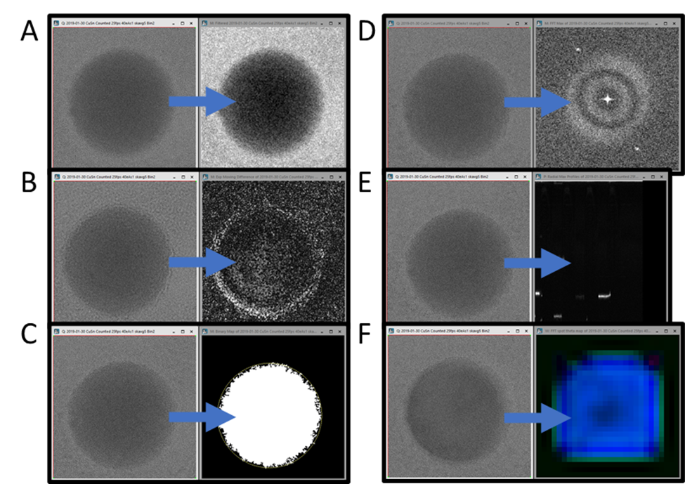
The first script reduces noise in the live view data using a gaussian blur or median filter (or both), as seen in Figure 1A. While it is possible to apply such processing to a single image using the standard DigitalMicrograph user interface, it is not possible to apply these in real-time to the live view, except via scripting. Since the Python package, SciPy, has these filters built-in, just a single line of code is required to apply one of these filters to the data. The output of this script is a new image the size of the ROI specified by the user, which updates as the live view updates. If no ROI is placed on the live view before running the script, an ROI is added that covers the entire image.

The simplest script is only a template and does not do any processing at all. It merely copies the data to a new window every time the data in the live view is updated. A comparison of the code in this script and the noise reduction script makes it even more clear which components should always be included and which can be modified to process the data in entirely different ways.

The following script produces a live difference display, making it easier to see where the intensity changes over time, as seen in Figure 1B. Simply subtracting the last frame from the current frame would produce a very noisy result. Instead, two exponentially weighted moving averages are computed (with two different time constants), and the absolute value of their difference is returned. Like the simple copy and noise reduction script, the output is an updating image of the size of the user-specified ROI. If the sample is drifting (as it usually does during in-situ experiments, then this difference display may be swamped by the effects of drift. Expansion of the data processing could try to align the images before averaging, or the script could be applied to data played back with the In-Situ Player after drift correction has been performed.

The last script that produces a processed image the same size and shape as the original, is shown in Figure 1C. This live thresholding with plots script thresholds the data and finds the largest contiguous bright region, placing a circular ROI on it. All the script details are beyond the scope of this application note. Still, an Otsu thresholding routine and some morphological operations are used to produce the binary image, followed by scikit-image-based measurement routines to find the center and convex area of the largest region. This script demonstrates one method for adding an updating annotation (here a circular ROI) to the image result in DigitalMicrograph. The script also demonstrates plotting data in an updating line plot. A video of the script running can be found on our Youtube channel: Real-time thresholding and tracking with Python in DigitalMicrograph.

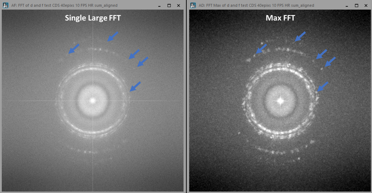
The following script (Live Max FFT) produces something like a diffractogram rather than a new real-space image, as shown in Figure 1D. Rather than simply performing a live fast Fourier transform (FFT) of the image, as DigitalMicrograph can already do easily, this script computes a “maximum FFT.” It does this by first dividing the image into many small regions and computing FFTs for each. Then instead of summing or averaging over all those FFTs, it finds the maximum so that each pixel in the result is the maximum over all the computed FFTs. The effect of this is to increase the signal from small crystalline regions which might otherwise be lost in the background intensity of a single large FFT, as shown in Figure 2, while decreasing the pixel resolution of the FFT.

The following script (Live Radial Profile) reduces the dimensionality of the input data, producing a 1D profile for each frame. Each profile is added as a column in the output image, so the horizontal axis is time, and the vertical axis is spatial frequency. The profiles produced by this script are radial profiles from FFTs of the input image frames. Again the full details of this processing are beyond the scope of this application note. Still, the result of this processing is that any changes in the crystallinity of the sample can be easily observed as a function of time. In Figure 1E, the sample repeatedly melted and crystallized in different orientations each time, so the output image shows this oscillation.

The final script in this collection (Live FFT Color Map) produces a color map of the crystalline regions of the sample. More details about how this is done can be found in the Magnetite nanoparticle orientation mapping from a single low-dose transmission electron microscope (TEM) image experiment brief on our website and the Direct visualization of the earliest stages of crystallization article published in Microscopy and Microanalysis. This script requires the most lines of custom Python code and relies on a module available on PyPI and can be installed via Pip (pip install BenMillerScripts). This is also the slowest of the scripts described here, with most of the time required to compute many FFTs from overlapping regions of the input image frames. However, even this script runs fast enough to provide useful feedback to the user during an experiment.

One additional feature of these live view processing scripts is that multiple scripts can be run concurrently. In Figure 3 below, a video demonstrates running all seven of these scripts simultaneously on a single dataset played back with the In-Situ player. Here the image frames are only 870 x 870 pixels since this was cropped from a much larger dataset, so processing each frame in all seven ways takes less than 1 s. 

Again, the primary purpose of these scripts is to serve as templates on which scripts specific to the applications of individual researchers can be based. Since Python is a well-known and powerful language for image processing and analysis and is also free, it should be accessible to many researchers who can modify these scripts to suit their needs. Introducing real-time data analysis during data acquisition will better inform crucial decision-making at the microscope.